The Dynamics of Market Forces—Squaring the Circle

By Carlos Fuentes

Understanding the applicability of supply and demand can help practicing actuaries not only analyze economic pricing but also assess the impact of tax policies, government intervention, and producer behavior.

---

Idea in Brief

• This article describes how economist Alfred Marshall synthesized the economic concepts that gave birth to the modern theory of pricing.
• The concepts of utility, supply, and demand are the basis of economic pricing.
• Supply-and-demand pricing relies on certain assumptions that are only approximately satisfied in the real world. Awareness of the degree of their accuracy, which is often lacking, helps assess the validity of economic models.
• Understanding the applicability of supply and demand, which varies by case, can be useful to the practicing actuary not only to assess economic pricing, but also to gauge the implications of tax policies, government intervention, and producer behavior.

---

This article connects the concepts discussed in “The Dynamics of Market Forces: Setting the Stage,” which appeared in the May/June issue of Contingencies, and describes the modern theory of supply and demand. It offers examples that show how the concepts of utility, supply, and demand are connected and how they determine the price of some (or many, depending on whether one believes the basic economic assumptions hold or not) goods and services.

The insights of the outstanding economists discussed in the previous article help clarify hypotheses that are often obscured by abstract mathematical formulations. In this context, the validity of the assumptions required to develop workable models is better understood through a historical perspective. The perspective reveals that, in some cases—such as those related to competition in the health care industry—the assumptions are less stable that it may seem.

This article explores the intricate dynamics of supply and demand, highlighting the complexities and limitations of applying these concepts in real-world scenarios. While supply-demand pricing offers valuable insights, it can fall short due to imperfect market conditions. The discussion extends to actuarial pricing, underscoring the challenges actuaries face in projecting costs and assessing risks. Ultimately, the article underscores the importance of understanding both the theoretical and practical aspects of pricing to navigate the economic landscape effectively.

Alfred Marshall^[1]

The main preoccupation of economic theory in the later part of the 19th century was to resolve the puzzle of value in use versus value in exchange. The breakthrough came in 1871 when Alfred Marshall, influenced by the work of several economists, including Carl Menger and William Stanley Jevons, postulated the following:

1. It is marginal utility, not total utility, that determines value: it is not the total satisfaction (the integral) from the possession and use of a product or service that gives it value; it is the satisfaction or enjoyment—the utility—from the last (derivative) and least wanted (because the utility curve slopes down) addition to one’s consumption that so serves. Thus, the price consumers are willing to pay (the demand) for a good or a service equals its marginal utility.

Consider the hypothetical total and marginal utilities of drinking water and wearing diamonds as represented by the following formulas and depicted in the graphs below:

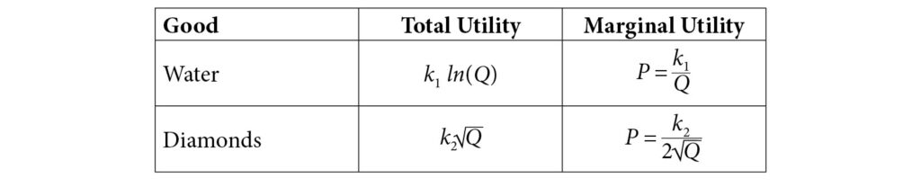
where

• Q is the quantity of the good under consideration in a suitable unit, say liters of water and ounces of diamonds;
• P is the price in dollars paid for a unit of the good under consideration;
• k₁ and k₂ are constants to be determined using econometric techniques.

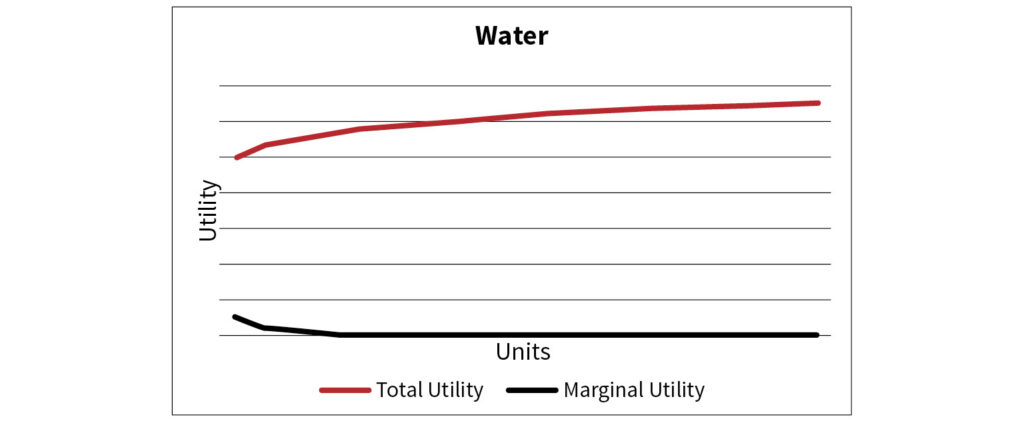
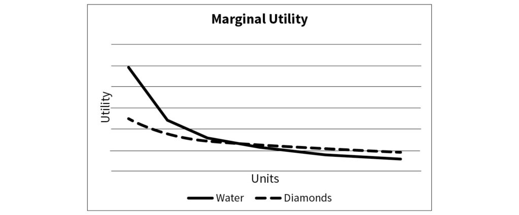
Consuming the first glass of water in a day yields a large utility because water is necessary to survive. The utility of consuming two glasses of water (the same day) is greater than the utility of consuming one but the increase in utility (from one to two glasses) is much smaller than the utility of consuming the first. The utility of consuming three glasses of water (the same day) is greater than that of consuming two but the increase in utility (from two to three glasses) is smaller than the increase from one to two, and much smaller than the utility of consuming the first glass. The argument can be continued for as long as there is water available. The process is illustrated in the Water graph in which the red line represents the (increasing) total utility and the black line the (decreasing) marginal utility.

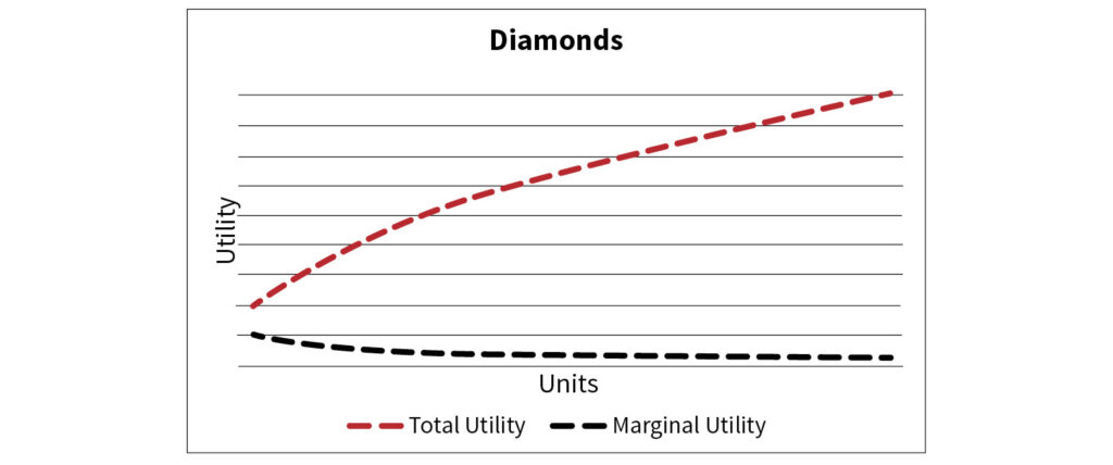
A similar argument can be made about diamonds. The Diamonds graph depicts their total and marginal utilities. As in the case of water, total utility is an increasing function whereas marginal utility is a decreasing function.

The Marginal Utility graph below compares marginal utilities and shows that the utility of additional units of water decreases faster than the utility of diamonds. The price (equal to the marginal utility) is what people are willing to pay for the last or least wanted increment. In other words, diminishing marginal utility leads to collectively reduced willingness to pay.

The demand of any good or service is commonly represented as a relationship of quantity (x-axis) and price (y-axis), although other variables can be involved. For example,

Q_d = a – bP + cM +dPR

where

• Q_d is the quantity demanded;
• P is the price of the good or service;
• M consumer income;
• PR is the price of a related good;
• a, b, c, d are constants.

These concepts will be illustrated with the demand functions of water and diamonds discussed above (not with the common linear relationship^[2]), that is, with

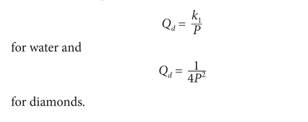
The demand of diamonds is more elastic (more sensitive to price) than the demand of water because diamonds are a luxury, not a necessity. The demand curves slope downward, showing the inverse relationship between price and quantity demanded—meaning that as an item becomes more expensive, fewer units will be sold.

2. At the same time, the rising marginal costs for producers and the higher costs for less efficient producers lead to increasing costs of additional supplies:^[3] the more that is sought, the more must be paid. This results in the ascending supply curve. The supply of any good is commonly represented with a linear relationship of quantity (x-axis) and price (y-axis) such as

Q_s = e + fP + gC

where

• Q_s is the quantity supplied;
• C is the cost of production;
• e, f, g are constants.

For illustrative purposes it will be assumed that the supply of water and diamonds are represented by

Q_s = c + dP

 for water and

Q_s = e + fP

for diamonds, where c = 0.5, d = 1.0, e = 15.0, f = 50, and, for the demand curves, k₁ = 1 k₂ =1.

The supply curves slope upward, reflecting the direct relationship between price and quantity supplied:

• The greater the price a producer can charge for a good, the more goods it will produce;
• The greater the slope in the equation (factors d, f), the more goods the seller will produce.

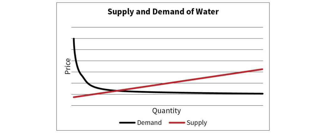
3. The point of intersection of the two curves determines the price necessary to induce the supply and the price that the least urgent need commands. For water, equating the quantities of water from the supply and demand curves results in

Thus, the price of water per liter is $1.64 = 1.28/0.78.

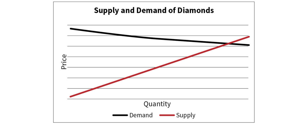
The two graphs, Supply and Demand of Water and Supply and Demand of Diamonds, illustrate the supply and demand curves for water and diamonds. Tradition dictates that quantity is the independent variable (a choice that may seem unnatural to non-economists) because, in some cases, price adjusts to quantity. Additionally, in certain economic analyses, such as calculating consumer surplus, producer surplus, and dead-weight loss,^[4] this choice of independent variable facilitates analysis and interpretation.

Value is the actual price once all the producers and consumers have had time to adjust their consumption and production to any changes in taste and/or technology. According to this theory, there is no difference between value and price. Since marginal cost is presumed to rise with output, the last unit produced is the costliest. Equilibrium is reached when marginal utility equals marginal cost, and both are equal to normal price.^[5]

Another requirement of this theory is that supply and demand forces be completely independent of each other so that the only connection between supply and demand is price. This typically does not pose a problem when studying the value of one good at a time.

Marshall’s theory of supply begins with work. Even if work is initially pleasant, it eventually becomes painful. The longer we work, the greater the discomfort; thus, the marginal disutility of labor is a function of time. Why does anyone work? Because, at first, wages more than compensate for the unpleasantness of labor. Why does anyone stop working? At some point, the wages offered no longer adequately compensate the worker for the fatigue of their labor. Therefore, a time-and-a-half rate for overtime labor presumably compensates the worker for the additional (marginal) fatigue.

Capital is also required to produce goods. The supply of both capital and labor depends on the discomfort that money payments can overcome. Marshall suggested that suitable rates of interest compensate savers for the increasing marginal discomfort of postponing pleasure.

Demand is the other side of the story. As we acquire more of anything, including money, the satisfaction it provides (its marginal utility) diminishes. Consequently, the price we are willing to pay for additional quantities decreases. The rational consumer is constantly engaged in a balancing act at the margin, continually comparing the additional satisfaction gained from spending on one good with the additional satisfaction that could be derived from an alternative purchase. In equilibrium, the hypothetical consumer concludes that no reallocation of her income could increase her satisfaction.^[6] A condition of equilibrium is the proportionality of prices to utilities.

The producer behaves like the consumer, comparing the additional output that $100 would yield when applied to labor, machines, better materials, or increased maintenance. Throughout, the principle of substitution guides the producer—both consumers and producers replace more expensive items with cheaper alternatives, optimizing their satisfaction or profit. This principle guides decision-making in economics.

Time is “the center of the chief difficulty of almost every economic problem.” How do prices behave over time? Marshall recognized the challenge of examining any concrete problem from a general equilibrium standpoint. To simplify the analysis, he introduced the concept of partial analysis. He asked his readers to imagine that we could focus on one industry and, within that industry, on a single business unit, the equally fictitious representative firm. “The forces to be dealt with are, however, so numerous that it is best to take a few at a time and to work out a number of partial solutions as auxiliaries to our main study.” Like many of his contemporaries, Marshall hoped to move from statics to dynamics, a goal that remains largely unfulfilled today.

How does time affect such an industry and such a firm? Employing another useful fiction Marshall identified three different time periods. Although these periods could be isolated only hypothetically^[7] and they shifted from problem to problem, they help us understand the events of real life.

1. The market period is the shortest of these time divisions, during which supplies are fixed, and demand determines price. Marshall carefully limited his demonstrations to relatively inexpensive, readily divisible items. Only in such cases could he plausibly assume that the marginal utility of money does not change for individual purchasers as they make successive purchases.
2. The short-run normal period lasts long enough for firms to adjust the supply of products manufactured in existing plants, though productive facilities remain constant and the law of diminishing returns^[8] applies. The forces that influence supply take a larger role. If consumer demand rises, producers expand output until the cost of the last unit of output produced equals its selling. Conversely, if demand falls, producers scale back production until the cost of the last unit matches the price received. If demand drops off significantly,theproducer may halt operations entirely.
3. In the long-run normal period, firms have sufficient time to expand their plants and adjust output from existing facilities. They can expand by adding new machines and constructing plant extensions to accommodate them. Additionally, older firms can exit the market while new firms enter. In modern terms, the law of returns to scale^[9] applies to all resources. What factors influence entrepreneurs as they make these decisions? When demand is too low to cover total costs, firms exit the market, leaving only those that can earn normal profits.^[10] If demand is extremely high, existing producers expand, and new producers enter the industry. In long-run equilibrium, prices cover all costs, including normal returns on capital. As this suggests, given enough time, supply—not demand—becomes the dominant force influencing price.

While these adjustments take place, many other factors come into play. As manufacturing becomes more specialized and machines replace human labor, the cost per unit of output shrinks. Education also plays a role, contributing to efficiency and innovation. Many industries benefit from increasing returns to scale, challenging the assumption of diminishing returns from land. In short, the pricing dynamics are complex, and many intricacies are often overlooked.

The price an individual pays for an item is equal to its marginal utility. According to the law of declining marginal utility, a consumer purchasing six units would have been willing to pay more for the first than the for the second, and so forth. The differences between what the consumer would have been willing to pay for all the six units and what the consumer actually paid constitutes consumer surplus. A discriminating monopolist, who charges different prices for different portions of sales, captures a portion of this surplus.

These conclusions have tax implications. An effective tax policy minimized the reduction of consumer surplus. By extension, this argument supports income taxes over commodity taxes, as income taxes allow consumers to adjust their spending in a way that minimizes the loss of surplus.

Can All Goods and Services Be Priced Using the Concepts of Supply and Demand?

The answer to this question is clearly no. Several conditions must be met for the effective application of supply and demand analysis, some of which have been discussed in the article. This section provides a summary of all these conditions:

1. Perfect Competition. This occurs in markets with numerous buyers and sellers, none of whom can influence prices. Products are homogeneous and information is freely available, ensuring that prices are determined purely by market forces.

2. Market Efficiency. In efficient markets, prices quickly reflect all available information. This transparency helps buyers and sellers to make informed decisions, aligning supply and demand more closely.

3. Elasticity of Supply and Demand. Both supply and demand should respond appropriately to price changes. If a product’s price drops, demand should increase, and vice versa, ensuring equilibrium pricing.

4. Absence of Externalities. Markets should operate without significant externalities, which are unaccounted costs or benefits to third parties. When externalities are present, prices may not reflect the true costs or benefits, requiring regulatory intervention. Examples of externalities include:

4.1
Factories that pollute without compensating society for the environmental damage they cause;

4.2
A company that provides training to employees, only for the employees to leave for another employer shortly after, without compensating the original company for training investment.

5. Minimal Government Intervention. When government regulations, subsidies, or price controls are minimal, prices are more likely to accurately reflect supply and demand dynamics.

6. Stable Economic Environment. A stable economy with predictable inflation and growth rates helps maintain consistent supply and demand, making market pricing more reliable.

7. Information Symmetry. Buyers and sellers should have access to the same information about the product or service, ensuring fair pricing based on true market conditions.

Due to space limitations, these conditions will not be analyzed in this article. However, it is clear that many of them are either not satisfied or only partially fulfilled in real markets. The extent to which these conditions are fulfilled impacts the accuracy of economic models in ways that are almost never quantified and often not even acknowledged. The unavoidable conclusion is that demand-supply pricing, like all economic constructs, is approximate and can lead—as it often does—to inaccurate results, even for goods and services that are important to society, and even when abundant data create the illusion of precision.

Actuarial Pricing

Traditional actuarial pricing is cost-driven, focusing on historical claim costs, expenses, and risk loads. Projecting claim costs can be challenging for reasons such as uncertainty and variability; benefit modifications (which can be particularly difficult to estimate in health care); evolving demographic; technological advancements such as new medical treatments; regulatory updates such as mandatory inclusion of benefits in a health care plan; economic factors such as inflation and unemployment rates (which can affect retirement rates) and; of course, data availability and quality. Risk loads can also be difficult to assess and include considerations such as marginal surplus requirements, expected profit, claims volatility, risk profile, and market dynamics.

Understanding economic pricing is still important for actuaries because it helps them assess the implications of issues such as tax policies and government intervention, and the national debates surrounding them. For example:

• What is meant by managed competition? Does the concept make sense in economics or is it simply a marketing slogan?
• Should fee-for-service competition in health care reward quality and cost-effectiveness while weeding out poor performers? If not, why not?
• Is government intervention beneficial in some circumstances? If so, under what conditions?
• What are the consequences of different tax policies?
• Are the salaries of executives, particularly in the health care industry, determined by impersonal market forces and therefore, objectively fair? 

Carlos Fuentes, MAAA, FSA, FCA, MBA, MS, is president of Axiom Actuarial Consulting. He can be reached at carlos-fuentes@axiom-actuarial.com.

Endnotes

1. Alfred Marshall (1842-1924) was a British economist and his most famous work, Principles of Economics, is one of the high points in the literature of social science. He was one of the founders of the school of Neoclassical Economics.
2. Note that Q_d in the linear equation is a decreasing linear function and its integral (the total utility) is an increasing function for P > 0. In other words, the total utility increases with Q and the marginal utility decreases with Q, as expected.
3. The supply curve can be a straight line when the following two conditions are satisfied: (1) there is perfect competition and production costs remain constant; (2) the marginal cost of production is constant. However, if marginal cost rises with output, the supply curve slopes upward.
4. A deadweight loss is a cost to society created by market inefficiency, which occurs when supply and demand are out of equilibrium. Mainly used in economics, deadweight loss can be applied to any deficiency caused by an inefficient allocation of resources.
5. Normal price is the outcome of permanent forces which bring about changes in demand and supply.
6. Individuals certainly engage in this type of decisions, which are normally driven by intuition or irrationality. The foregoing notwithstanding, economics dogmatism postulates rationality.
7. In many cases it is assumed that these periods are well defined, which is certainly not the case.
8. The law of diminishing returns states that as more units of a variable input are added to a fixed input, the additional output produced from each new unit will eventually decrease.
9. The law of returns to scale states that as all inputs are increased proportionally, the resulting output will increase at a constant, increasing, or decreasing rate, depending on the scale.
10. Under normal profits, a firm makes sufficient revenue to cover its total costs and remain competitive in an industry. Normal profits factor in the opportunity cost—the value of the best alternative forgone. When a firm makes normal profit we say the economic profit is zero.